How to Use
The following are helpful tutorials for using the mapping package.
While best to follow in order, each section does not neccessarily have to rely on the ones before.
For interactive tutorials, checkout the Jupyter notebooks in tutorials/.
Units
When passing in arguments that have a unit associated with it, there exists default units but specific units can also be passed.
>>> import scanning
>>>
>>> # using astropy
>>> import astropy.units as u
>>> mod = scanning.Module(wavelength=0.0005*u.m)
>>>
>>> # using strings
>>> mod = scanning.Module(wavelength='0.0005 m')
When receiving values that have an associated unit, typically by accessing a property of the object, an astropy.units.Quantity object is returned. You can convert to a specific unit in a similar way.
>>> print(mod.ang_res)
>>> print(mod.ang_res.to(u.arcsec).value))
>>> print(mod.ang_res.to('arcsec').value))
0.005733544455586236 deg
20.64076004011045
20.64076004011045
See astropy.units for a list of unit names that you can use. Notable ones include:
- angle-like:
arcmin/arcminute
arcsec/arcsecond
deg/degree(usually the default)
hourangle
rad/radian
- time-like:
h/hour/hr
min/minute
s/second(usually the default)
Building Modules and Instruments
The Module class allows one to represent a camera module, which consists of three wafers each consisiting of three rhombuses.
You can create a Module object by passing an F_Lambda and wavelength or freq.
>>> import scanning
>>> mod = scanning.Module(freq=400, F_lambda=1.2)
There are also pre-defined Module objects, all at 1.2 F-Lambda, that you can import from scanning:
SFH- 860 GHz
CMBPol- 350 GHz
EoRSpec- 262.5, 262.5, and 367.5 GHz (one for each wafer)
Mod280- 280 GHz
You can save this module as a csv file by specifying which columns you would like to save. You can also specify the units you would like to save in. To return the data as a dictionary, do not specify a path in the first argument.
>>> # save as a csv file with specific columns and units
>>> mod.save_data('sample_module.csv', columns={'x': 'arcsec', 'y': 'arcsec', 'pol': 'deg', 'rhombus': None, 'wafer': None})
>>>
>>> # return a dictionary (units by default are in degrees)
>>> mod.save_data(columns=['x', 'y'])
{'x': [0.3398681466571475, 0.34416533012062867, 0.34846251358410985,...
To re-generate the same object, pass that csv file or dictionary into Module.
Note that all columns (x, y, pol, rhombus, wafer) are recommended to be passed.
>>> scanning.Module('sample_module.csv', units={'x': 'arcsec', 'y': 'arcsec', 'pol': 'deg'})
The Instrument class (with PrimeCam and
ModCam being specific subclasses) allows one to
configure multiple Module objects into any location relative to the boresight.
You can fill up an Instrument with Module objects and specify its location in polar coordinates and rotation.
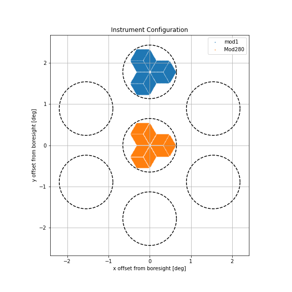
>>> prime_cam = scanning.PrimeCam()                                    # empty Instrument
>>> prime_cam.add_module(mod, location=(1.78, 90), identifier='mod1') # location in terms of (dist, theta)
>>> prime_cam.add_module(mod, location='i1', identifier='mod2')       # location in terms of a pre-defined slot
>>> prime_cam.add_module('Mod280', location='i2')                      # a pre-defined module str option
You can also change modules and delete modules.
>>> prime_cam.change_module('Mod280', new_location=(0, 0))
>>> prime_cam.change_module('mod2', new_identifier='mod2_renamed')
>>> prime_cam.delete_module('mod2_renamed')
>>> prime_cam
instrument: offset [0. 0.] deg, rotation 0.0 deg
------------------------------------
mod1
 (r, theta) = (1.78, 90), rotation = 0.0
Mod280
 (r, theta) = (0.0, 0.0), rotation = 0.0
Using scanning.visualization.instrument_config(), this is what the instrument looks like:
Slot names such as ‘i1’ or ‘c’, , which are different for each subclass, can get queried like so:
>>> prime_cam.slots
{'c': <Quantity [0., 0.] deg>,
 'i1': <Quantity [  1.78, -90.  ] deg>,
 'i2': <Quantity [  1.78, -30.  ] deg>,
 'i3': <Quantity [ 1.78, 30.  ] deg>,
 'i4': <Quantity [ 1.78, 90.  ] deg>,
 'i5': <Quantity [  1.78, 150.  ] deg>,
 'i6': <Quantity [   1.78, -150.  ] deg>}
You can save this Instrument object’s data as a json file (or dictionary if no path is specified).
It will contain the instr_offset, instr_rot, and all info about each Module object.
To re-generate the same Instrument object, pass that json file or dictionary into the constructor.
>>> prime_cam.save_data('PrimeCam.json')
>>> scanning.PrimeCam('PrimeCam.json')
Representing Scan Patterns
It is useful to represent the path of the detector array on the sky.
SkyPattern can represent the RA/DEC offsets of an arbitray pattern, which can be used on any source.
Daisy is a specific example of such a pattern and is optimized for point sources.
There is also the Pong pattern, which is are optimized for regions a few square degrees.
Pass in appropriate parameters to generate a pattern.
>>> import scanning
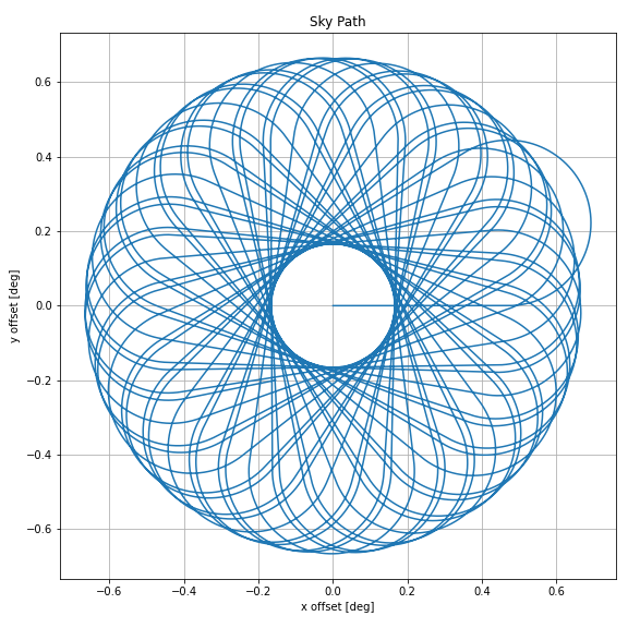
>>> daisy = scanning.Daisy(velocity=1/3, start_acc=0.2, R0=0.47, Rt=800*u.arcsec, Ra=600*u.arcsec, T=300, sample_interval=1/400)
Using scanning.visualization.sky_path(), this is what the above pattern looks like in RA/DEC offsets.
Those parameters can then be saved as a json file (or returned as a dictionary if no path is specified) and passed into the constructor to re-generate the same pattern. Use keyword arguments to overwrite specific parameters.
>>> daisy.save_param('sample_daisy.json')
>>> scanning.Daisy('sample_daisy.json', Ra=1200*u.arcsec)
You can also save the data as a csv file and specify desired units and columns.
Note that if done this way, information about the parameters are not saved,
so this csv file cannot be passed into the same subclass constructor (such as Daisy or Pong).
Instead, you can pass the csv file or dictionary (so long as “time_offset”, “x_coord”, and “y_coord” are columns) into the SkyPattern constructor.
>>> daisy.save_data('sample_sky_pattern.csv', columns={'time_offset': 's', 'x_coord': 'arcsec', 'y_coord': 'arcsec'})
>>> scanning.SkyPattern('sample_sky_pattern.csv', units = {'time_offset': 's', 'x_coord': 'arcsec', 'y_coord': 'arcsec'})
A TelescopePattern stores time offset, sidereal time, azimuth coordinates, and elevation coordinates.
Typically, this can be interpreted as the path of the boresight for a particular scan,
but that does not neccessarily have to be the case.
One way of intializing a TelescopePattern is by passing a SkyPattern instance along with observational
data that has the right ascension and declination of your source, and some way to initialize time.
Optionally, you can pass an Instrument object and choose a module where the SkyPattern is applied to.
The module parameter data_loc can be a slot location, module identifier, or a (dist, theta).:
t = scanning.TelescopePattern(
    daisy, instrument=scanning.PrimeCam(), data_loc='i1',
    start_ra=60, start_dec=-60, start_elev=40, moving_up=True
)
There are a few parameters (that are mutually exclusive) that can be used to initialize a start time:
start_datetime
start_hrang(hour angle)
start_lst(local sidereal time)
start_elevandmoving_up(default True)
Similar to SkyPattern, you can save the parameters of observation to use later on.
>>> t.save_param('sample_tp_param.json')
>>> scanning.TelescopePattern(daisy, scanning.PrimeCam(), data_loc='i1', obs_param='sample_tp_param.json')
Now that you have an initialized TelescopePattern, suppose you want to see any module away from the boresight.
The following returns a new TelescopePattern where the stored AZ/EL coordinates are that of the specified module.
Note that this new object does not retain instrument information, since the idea of a boresight is not applicable anymore.
>>> t_i5 = t.view_module('i5')
You can also get the corresponding SkyPattern object.
In the example below, this would get a SkyPattern object representing the x-y offsets made by slot “i5”.
>>> t_i5.get_sky_pattern()
Similar to SkyPattern, you can save the data as a csv file (or return the data as a dictionary) and pass it into the constructor to initialize it again.
You can specify columns and units you would like to save. See docstrings for more information.
>>> t.save_data('sample_tp.csv', columns={'time_offset': 's', 'lst': 'deg', 'az_coord': 'deg', 'alt_coord': 'deg'})
>>> scanning.TelescopePattern('sample_tp.csv', units={'time_offset': 's', 'lst': 'deg', 'az_coord': 'deg', 'alt_coord': 'deg'})
Simulating Scan Patterns
See tutorial Jupyter notebook.
Optimal Observation Times
An Observation object represents an observation of a source(s) for a particular time range, and can be used to find the ideal time for observation.
You can pass a list of declinations. By default, the observation period is the full 24 hour angle range. You can see when the object fits certain conditions (and return this information).
>>> obs = scanning.Observation([30, 0, -20])
>>> obs.filter(min_elev=30, max_elev=75, min_rot_rate=15)
(dec=30.0N):  [[-0.5279999999999898, 1.9520000000000124]]
(dec=0.0N):  [[-1.1039999999999903, 3.792000000000014]]
(dec=-20.0N):  [[-4.319999999999993, -2.6079999999999917], [1.0560000000000116, 1.7280000000000122]]
Other than hour angle, you can pass a datetime range instead. Corresponding right ascension(s) must also be listed.
>>> scanning.Observation([30, 0, -20], datetime_range=['2001-12-09', '2001-12-10'], ra=[0, 2, 4]*u.hourangle)